
You have a spreadsheet full of sales data, expenses, or inventory numbers. You need to add up only the values that match a specific condition, say all sales from one particular salesperson, or all expenses above a certain amount. You could scroll through row by row and add things manually, but that would take forever and leave room for mistakes.
This is exactly the problem the SUMIF Function in Excel was built to solve. It lets you add up values automatically based on a condition you set. Instead of manually filtering and summing, you write one formula, and Excel does all the work in a fraction of a second.
Table of Contents
Whether you are a student managing a budget, a small business owner tracking sales, or a professional analyzing data, mastering SUMIF Excel will save you hours of work and make your spreadsheets dramatically more powerful. This guide explains everything from scratch, with clear examples you can follow right away.
What Is the SUMIF Function in Excel?
The SUMIF Function in Excel is a formula that adds up numbers in a range only when they meet a specific condition. Think of it as a combination of two things: SUM, which adds numbers, and IF, which checks a condition. Put them together and you get SUMIF add numbers only if a condition is true.
Here is a simple real-world example. Imagine you run a small shop and you have a spreadsheet with a list of products in one column and their sales amounts in another column. You want to know the total sales for just one product, say, “Coffee.” Instead of scrolling through hundreds of rows and adding them up manually, you use the SUMIF Function to find every row that says “Coffee” and add up only those sales values automatically.
The result appears instantly, and if new Coffee sales get added to the spreadsheet later, the formula updates automatically.
Understanding the SUMIF Syntax
Before writing your first formula, you need to understand how it is structured. Every SUMIF Function in Excel has three parts.
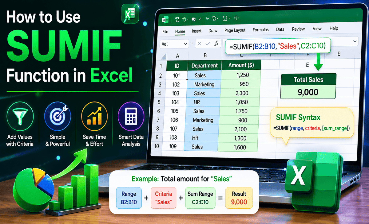
=SUMIF(range, criteria, sum_range)Here is what each part means.
Range is the group of cells Excel looks through to check your condition. In the coffee example, this would be the column listing product names.
Criteria is the condition you want to match. This could be a word like “Coffee,” a number like 100, or a comparison like “>50” (meaning greater than 50).
Sum_range is the column of numbers you want to add up when the condition matches. In the coffee example, this would be the column containing the sales amounts.
If your sum_range is the same as your range meaning the numbers you want to add are in the same column you are checking you can actually leave the third argument out. But in most practical uses, you will have separate columns for your condition and your numbers.
Step-by-Step: Your First SUMIF Formula
Let us walk through building a SUMIF Formula from the ground up using a clear example.
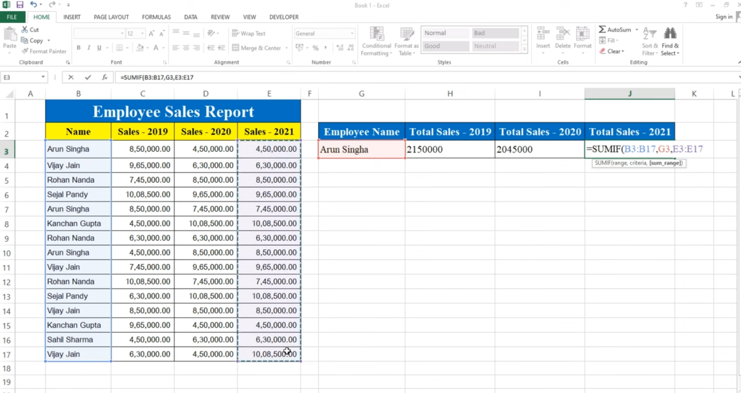
Imagine you have a spreadsheet tracking your team’s sales. Column A contains the salesperson’s name, column B contains the product they sold, and column C contains the sale amount. Your data starts at row 2 and goes to row 11.
Step 1: Click on an empty cell where you want your result to appear. Let us say cell F2.
Step 2: Type an equals sign to start the formula:
=SUMIF(
Step 3: Select your range the column you want Excel to search through. Since you want to find all sales by a specific person, click and drag to select A2 through A11. Your formula now looks like:
=SUMIF(A2:A11,
Step 4: Type your criteria the value you want to match. If you want to add up sales for “Sarah,” type her name in quotes:
=SUMIF(A2:A11,"Sarah",
Step 5: Select your sum_range the column with the numbers you want to add. Click and drag to select C2 through C11:
=SUMIF(A2:A11,"Sarah",C2:C11)
Step 6: Close the parenthesis and press Enter.
Excel instantly calculates the total sales for Sarah only, ignoring every other salesperson. That is SUMIF Excel in action.
Using Cell References Instead of Typing Criteria
Typing the criteria directly in the formula works, but there is a smarter way. Instead of typing “Sarah” inside the formula, you can reference a cell that contains the name. This makes your spreadsheet far more flexible.
For example, if you type “Sarah” in cell F1, your formula in F2 becomes:
=SUMIF(A2:A11,F1,C2:C11)
Now, if you change F1 to “James,” the formula automatically updates to show James’s total instead. This is especially useful when you want to create a dropdown or a simple lookup dashboard where changing one cell updates multiple results.
SUMIF With Number Conditions
The SUMIF Function in Excel is not just for matching text. It is equally powerful with numbers and comparisons. Here are the most common comparison operators you can use in your criteria.
Use > for greater than. Use < for less than. Use >= for greater than or equal to. Use <= for less than or equal to. Use <> for not equal to.
Example: To add up all sales amounts in C2:C11 that are greater than 500, you would write:
=SUMIF(C2:C11,">500")
Notice that in this case, the range and sum_range are the same column, so you only need two arguments.
Example: To add up all sales amounts that are 1000 or less:
=SUMIF(C2:C11,"<=1000")
These comparison criteria must always be enclosed in quotes, even though they involve numbers.
Using Wildcards in SUMIF Excel
Wildcards let you match partial text, which is incredibly useful when your data is not perfectly consistent or when you want to match a group of items that share a word.
The asterisk * matches any number of characters. The question mark ? matches exactly one character.
Example: You have a list of product names and some are “Coffee Latte,” “Coffee Black,” and “Coffee Mocha.” To add up all coffee sales regardless of the specific type:
=SUMIF(B2:B11,"Coffee*",C2:C11)
The asterisk tells Excel to match anything that starts with “Coffee,” no matter what comes after it.
Example: If you want to match any product that ends with “Latte”:
=SUMIF(B2:B11,"*Latte",C2:C11)
Wildcards make SUMIF much more flexible when dealing with real-world, slightly messy data.
SUMIF With Date Conditions
Dates work in SUMIF Excel too, which makes it useful for time-based reports like monthly summaries or date range analysis.
Example: To add up all sales from before January 1, 2025:
=SUMIF(D2:D11,"<01/01/2025",C2:C11)
Here D2:D11 contains dates and C2:C11 contains the corresponding sale amounts. You can also combine SUMIF with the DATE function for more precision:
=SUMIF(D2:D11,"<"&DATE(2025,1,1),C2:C11)
Using the ampersand & joins the comparison operator with the DATE function result, which is a cleaner approach when building dynamic date conditions.
Practical Tips for Using SUMIF Function
Here are some real-world tips that will help you use SUMIF more effectively and avoid common mistakes.
First, always lock your ranges with absolute references if you plan to copy the formula to other cells. Add a dollar sign before the column letter and row number, like $A$2:$A$11, so the range does not shift when you drag the formula. Also, remember that SUMIF is not case-sensitive; it treats “Sarah,” “sarah,” and “SARAH” as identical. If you need a case-sensitive match, you will need a more advanced array formula. Keep your criteria column clean and consistent because extra spaces before or after text can cause SUMIF to miss matches. Use the TRIM function to clean up messy data before relying on SUMIF formulas.
Another useful tip is to use named ranges instead of cell references like A2:A11, as they make formulas easier to read and understand. For example, naming your sales column “SalesAmount” lets you write =SUMIF(SalesRep,”Sarah”,SalesAmount). If you need to sum values based on multiple conditions, such as sales by Sarah and only for Coffee, upgrade to the SUMIFS function. It works similarly to SUMIF but allows you to apply two or more criteria at the same time, making it more powerful for complex data analysis.
Comparison: SUMIF vs SUM vs SUMIFS
Understanding when to use SUMIF versus its close relatives saves time and confusion.
SUM adds everything in a range with no conditions. Use it when you want a total of all values.
SUMIF adds values that meet one condition. Use it when you have a single rule to apply.
SUMIFS adds values that meet two or more conditions simultaneously. Use it when your filtering needs multiple rules at once.
For example, if you want total sales where the salesperson is “Sarah” AND the product is “Coffee,” SUMIF alone cannot handle two conditions at the same time that is when SUMIFS steps in.
FAQ
What is the SUMIF Function in Excel used for?
The SUMIF Function in Excel adds up numbers in a range only when they match a specific condition. It is used to calculate conditional totals for example, total sales for one product, total expenses above a certain amount, or total revenue from a specific region.
Why is my SUMIF formula returning zero?
A zero result usually means the criteria did not match anything in the range. Common reasons include extra spaces in the cells, mismatched data types (such as numbers stored as text), or a typo in the criteria. Double-check that your range, criteria, and sum_range all refer to the correct columns and that your criteria exactly matches the data.
Can I use SUMIF with multiple conditions?
Not directly. The SUMIF Function supports only one condition. For two or more conditions, use the SUMIFS Function, which accepts multiple range and criteria pairs and adds values that match all of them simultaneously.
Does SUMIF Excel work with dates?
Yes. You can use date comparisons as criteria in SUMIF, such as ">01/01/2025" or combined with the DATE function for precision. Make sure the cells containing dates are formatted as dates and not stored as text, or the comparison may not work correctly.
Is the SUMIF Function case-sensitive?
No. SUMIF Excel treats uppercase and lowercase letters as the same. “apple,” “Apple,” and “APPLE” all match each other. If you need a case-sensitive match, you need to use an array formula with SUMPRODUCT and EXACT instead.
Conclusion
The SUMIF Function in Excel is one of the most practical and time-saving formulas you can learn. Once you understand its three-part structure range, criteria, and sum_range you can apply it to almost any situation where you need conditional totals.
Whether you are tracking sales, managing a budget, analyzing inventory, or summarizing expenses, SUMIF Excel gives you instant answers without manual sorting or filtering. Add wildcards for partial matches, use comparison operators for number and date conditions, and reference cells for flexible, dynamic formulas.
Start with the simple examples in this guide, practice on your own data, and you will quickly discover how often this one formula solves problems that used to take minutes or hours by hand.
The SUMIF Function is not just a formula it is a productivity upgrade for every spreadsheet you will ever build.